深度学习(4-5节)
多层的深层神经网络
神经网络的表示
1.L代表神经网络的层数(layers),不包括输入层,比如一个4层网络称为L-4
2.$n^{[l]}$代表$l$层上节点的数量,也可以说是隐藏单元的数量
3.$a^{[l]}$代表$l$层中的激活函数,$a^{[l]}=g^{[l]}(z^{[l]})$
深层网络中的前向传播
神经网络中每层的前向传播过程:
$$
Z^{[l]}=W^{[l]}a^{[l-1]}+b^{[l]}\
a^{[l]}=g^{[l]}(z^{[l]})\
l代表层数
$$
如果需要计算前向传播的层数过多,可以使用for循环将它们串起来。
核对矩阵中的维数
如果我们在实现一个非常复杂的矩阵时,需要特别注意矩阵的维度问题。
通过一个具体的网络来手动计算一下维度:
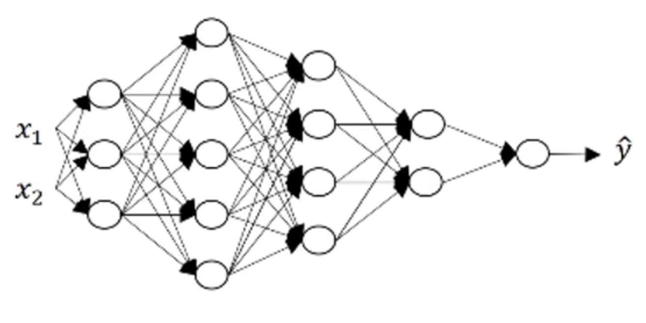
可以写出该网络的部分参数如下:
$$
n^{[0]}=n_x=2\quad n^{[1]}=3\quad n^{[2]}=5\quad n^{[3]}=4\quad n^{[4]}=2\quad n^{[5]}=1
$$
由于前向传播的公式为:
$$
Z^{[l]}=W^{[l]}a^{[l-1]}+b^{[l]}\
a^{[l]}=g^{[l]}(z^{[l]})
$$
需要说明的是这里的维度都是只在一个样本的情况下。如果在m个样本的情况下,1都要变成m,但b的维度可以不变,因为通过python中的广播技术,b会自动扩充。
1.$b^{[1]}$的维度为$3\times 1$,所以$Z^{[1]}$的维度也是一样的,为$n^{[1]}\times 1$也就是$3\times 1$。
2.$X$的维度为$n^{[0]}\times 1$,也就是$2\times 1$
所以通过1,2两条可以推出$W^{[1]}$的维度为$n^{[1]}\times n^{[0]}$,也就是$3\times 2$。
可以总结出来的是:
$$
W^{[l]}的维度一定是n^{[l]}\times n^{[l-1]}\
b^{[l]}的维度一定是n^{[l]}\times 1
$$
同理在反向传播时:
$$
dW和W的维度必须保持一致,db必须和b保持一致
$$
因为$Z^{[l]}=g^{[l]}(a^{[l]})$,所以$z$和$a$的维度应该相等。
参数vs超参数
参数(Parameters):$W^{[1]},b^{[1]},W^{[2]},b^{[2]},\dots$
超参数:学习率$a$;迭代次数$i$ ;隐层数$L$;隐藏单元数$n^{[l]}$;激活函数的选择。
作业三
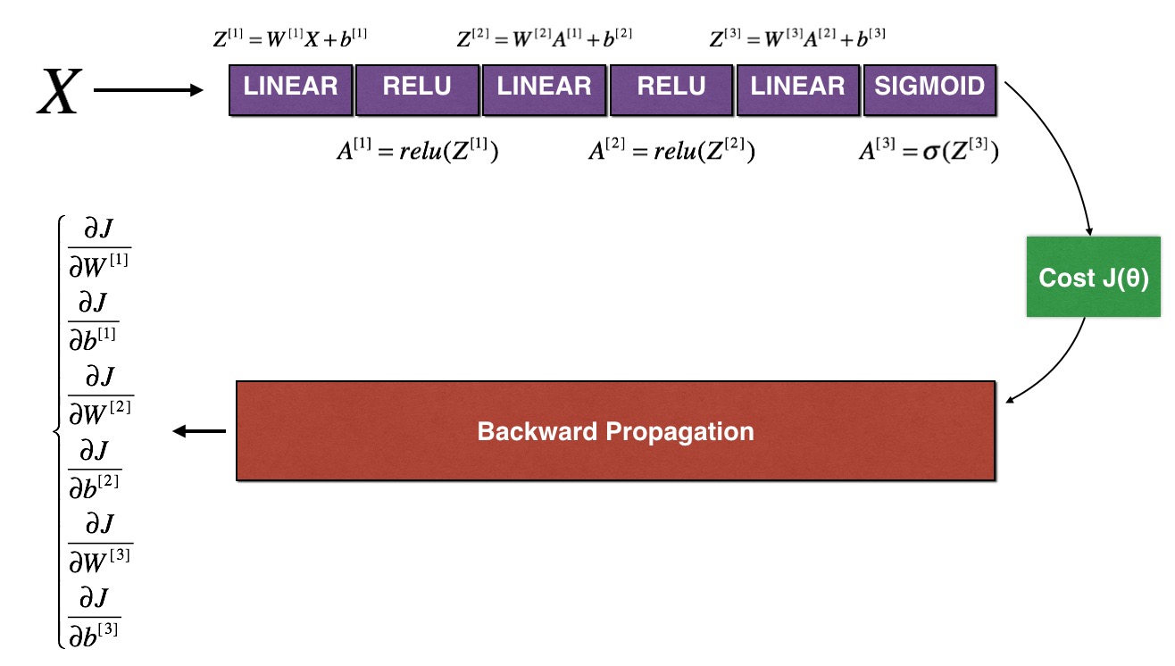
一个神经网络工作原理的模型如下:
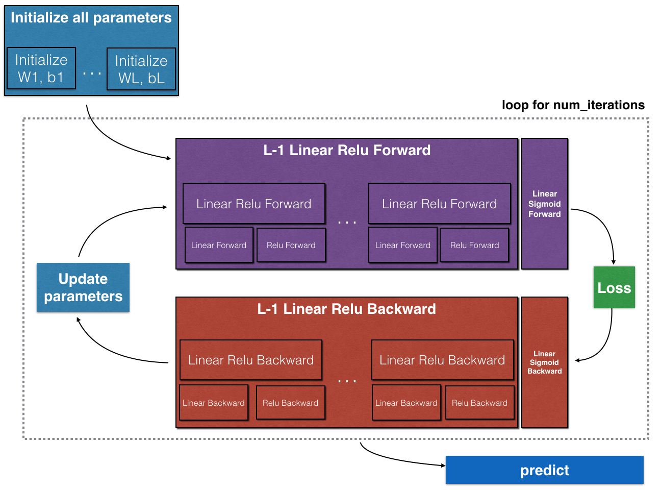
多层网络模型的前向传播和后向传播过程如下:
  1
  2
  3
  4
  5
  6
  7
  8
  9
 10
 11
 12
 13
 14
 15
 16
 17
 18
 19
 20
 21
 22
 23
 24
 25
 26
 27
 28
 29
 30
 31
 32
 33
 34
 35
 36
 37
 38
 39
 40
 41
 42
 43
 44
 45
 46
 47
 48
 49
 50
 51
 52
 53
 54
 55
 56
 57
 58
 59
 60
 61
 62
 63
 64
 65
 66
 67
 68
 69
 70
 71
 72
 73
 74
 75
 76
 77
 78
 79
 80
 81
 82
 83
 84
 85
 86
 87
 88
 89
 90
 91
 92
 93
 94
 95
 96
 97
 98
 99
100
101
102
103
104
105
106
107
108
109
110
111
112
113
114
115
116
117
118
119
120
121
122
123
124
125
126
127
128
129
130
131
132
133
134
135
136
137
138
139
140
141
142
143
144
145
146
147
148
149
150
151
152
153
154
155
156
157
158
159
160
161
162
163
164
165
166
167
168
169
170
171
172
173
174
175
176
177
178
179
180
181
182
183
184
185
186
187
188
189
190
191
192
193
194
195
196
197
198
199
200
201
202
203
204
205
206
207
208
209
210
211
212
213
214
215
216
217
218
219
220
221
222
223
224
225
226
227
228
229
230
231
232
233
234
235
236
237
238
239
240
241
242
243
244
245
246
247
248
249
250
251
252
|
from dnn_utils_v2 import sigmoid, sigmoid_backward, relu, relu_backward
import numpy as np


# ------------------------------------------
def initialize_parameters_deep(layer_dims):
    """
    Arguments:
    layer_dims -- 包含网络中每一层的维度的Python List

    Returns:
    parameters -- Python参数字典 "W1", "b1", ..., "WL", "bL":
                    Wl -- weight matrix of shape (layer_dims[l], layer_dims[l-1])
                    bl -- bias vector of shape (layer_dims[l], 1)
    """

    np.random.seed(3)
    parameters = {}
    L = len(layer_dims) # 网络层数

    for i in range(1, L):
        parameters["W" + str(i)] = np.random.randn(layer_dims[i], layer_dims[i - 1]) * 0.01
        parameters["b" + str(i)] = np.zeros(layer_dims[i], 1)

        assert(parameters["W" + str(i)].shape == (layer_dims[i], layer_dims[i - 1]))
        assert(parameters["b" + str(i)].shape == (layer_dims[i], 1))

    return parameters

# ------------------------------------------
def linear_forward(A, W, b):
    """
    实现前向传播的线性部分

    Arguments:
    A -- 来自上一层的激活结果 (或者为初始输入数据): (前一层的隐藏单元数, 样本数)
    W -- 权重矩阵: numpy array of shape (当前层的隐藏单元数, 前一层的隐藏单元数)
    b -- 偏置向量, numpy array of shape (当前层的隐藏单元数, 1)

    Returns:
    Z -- 激活函数的输入或称为预激活参数
    cache -- Python参数字典包含"A", "W" and "b" ; stored for computing the backward pass efficiently
    """

    Z = np.dot(W, A) + b

    assert(Z.shape == (W.shape[0], A.shape[1]))

    cache = (A, W, b)

    return Z, cache

# ------------------------------------------
def linear_activation_forward(A_prev, W, b, activation):
    """
    实现 线性——>激活层 的前向传播

    Arguments:
    A_prev -- 来自上层的激活结果 (或为初始输入数据): (前一层的隐藏单元数, 样本数)
    W -- 权重矩阵: numpy array of shape (当前层的隐藏单元数, 前一层的隐藏单元数)
    b -- 偏置向量, numpy array of shape (当前层的隐藏单元数, 1)
    activation -- 当前隐藏层使用的激活函数: "sigmoid" or "relu"

    Returns:
    A -- 激活函数的输出,也称为激活后值
    cache -- Python字典包含 "线性缓存" and "激活缓存";
             stored for computing the backward pass efficiently
    """

    if activation == "sigmoid":
        Z, linear_cache = linear_forward(A_prev, W, b)
        A, activation_cache = sigmoid(Z)

    elif activation == "relu":
        Z, linear_cache = linear_forward(A_prev, W, b)
        A, activation_cache = relu(Z)

    assert(A.shape == (W.shape[0], A.shape[1]))
    cache = (linear_cache, activation_cache)

    return A, cache

# ------------------------------------------
# 为了实现L层神经网络更加方便,需要将前L-1层的激活函数设置为ReLU,最后一层输出层激活函数设置为Sigmoid
def L_model_forward(X, parameters):
    """
    实现前向传播: the [LINEAR->RELU]*(L-1)->LINEAR->SIGMOID computation

    Arguments:
    X -- 初始数据, numpy array of shape (输入层大小, 样本数量)
    parameters -- 初始化deep网络的参数输出

    Returns:
    AL -- 上一层激活后的值
    caches -- cache的列表:
                every cache of linear_relu_forward() (there are L-1 of them, indexed from 0 to L-2)
                the cache of linear_sigmoid_forward() (there is one, indexed L-1)
    """

    caches = []
    A = X
    L = len(parameters) // 2
    # 前L-1层为relu激活函数
    for i in range(1, L):
        A_prev = A
        A, cache = linear_activation_forward(A_prev, parameters["W" + str(i)], parameters["b" + str(i)], "relu")
        caches.append(cache)
    # 最后一层为sigmoid激活函数
    AL, cache = linear_activation_forward(A, parameters["W" + str(L)], parameters["b" + str(L)], "sigmoid")
    caches.append(cache)

    assert(AL.shape == (1, X.shape[1]))

    return AL, caches

# ------------------------------------------
def compute_cost(AL, Y):
    """
    计算代价函数 使用Logistic回归中使用的代价函数

    Arguments:
    AL -- 对应于标签的预测概率向量, shape (1, 样本数)
    Y -- 正确的样本 (for example: containing 0 if non-cat, 1 if cat), shape (1, 样本数)

    Returns:
    cost -- 交叉熵代价
    """

    m = Y.shape[1]
    cost = -(np.dot(np.log(AL), Y.T) + np.dot(np.log(1 - AL), (1 - Y).T)) / m

    cost = np.squeeze(cost) # 使得cost的维度是我们想要的(比如将[[17]]变成17)
    assert(cost.shape == ())

    return cost

# ------------------------------------------
def linear_backward(dZ, cache):
    """
    单层实现反向传播的线性部分(l层)

    Arguments:
    dZ -- 代价函数对于线性输出的梯度 (l层)
    cache -- 元组(A_prev, W, b) 来自当前层的前向传播

    Returns:
    dA_prev -- 代价函数对于激活的梯度(l-1层), 和A_prev相同的维度
    dW -- 代价函数对于W的梯度 (l层), 和W相同的维度
    db -- 代价函数对于b的梯度 (l层), 和b相同的维度
    """

    A_prev, W, b = cache
    m = A_prev.shape[1]

    dW = np.dot(dZ, A_prev.T) / m
    db = np.sum(dZ, axis=1, keepdims=True) / m
    dA_prev = np.dot(W.T, dZ)

    assert(dA_prev.shape == A_prev.shape)
    assert(dW.shape == W.shape)
    assert(db.shape == b.shape)

    return dA_prev, dW, db

# ------------------------------------------
def linear_activation_backward(dA, cache, activation):
    """
    实现 线性——>激活 过程的反向传播

    Arguments:
    dA -- 当前层l激活后的梯度
    cache -- 元组 (linear_cache, activation_cache) 为了有效计算后向传播而存储
    activation -- 当前层的激活函数, stored as a text string: "sigmoid" or "relu"

    Returns:
    dA_prev -- 代价函数对于激活的梯度(l-1层), 和A_prev相同的维度,和A_prev相同的维度
    dW -- 代价函数对于W的梯度 (l层), 和W相同的维度
    db -- 代价函数对于b的梯度 (l层), 和b相同的维度
    """

    linear_cache, activation_cache = cache

    if activation == "relu":
        dZ = relu_backward(dA, activation)
        dA_prev, dW, db = linear_backward(dZ, linear_cache)

    elif activation == "sigmoid":
        dZ = sigmoid_backward(dA, activation_cache)
        dA_prev, dW, db = linear_backward(dZ, linear_cache)

    return dA_prev, dW, db

# ------------------------------------------
def L_model_backward(AL, Y, caches):
    """
    前L-1层为ReLU激活函数,最后一层为sigmoid函数的后向传播实现

    Arguments:
    AL -- 前向传播输出的概率向量 (L_model_forward())
    Y -- 真实值的向量 (containing 0 if non-cat, 1 if cat)
    caches -- 包含cache的列表:
                every cache of linear_activation_forward() with "relu" (it's caches[l], for l in range(L-1) i.e l = 0...L-2)
                the cache of linear_activation_forward() with "sigmoid" (it's caches[L-1])

    Returns:
    grads -- 带有渐变值的字典
             grads["dA" + str(l)] = ...
             grads["dW" + str(l)] = ...
             grads["db" + str(l)] = ...
    """

    grads = {}
    L = len(caches)
    m = AL.shape[1]
    Y = Y.reshape(AL.shape) # 经过这一行转化,Y的维度和AL维度相同

    dAL = -(np.divide(Y, AL) - np.divide(1 - Y, 1 - AL))

    current_cache = caches[L - 1]
    grads["dA" + str(L)], grads["dW" + str(L)], grads["db" + str(L)] = linear_activation_backward(dAL, current_cache, activation="sigmoid")

    for i in reversed(range(L-1)):
        current_cache = caches[i]
        dA_prev_temp, dW_temp, db_temp = linear_activation_backward(grads["dA" + str(i + 2)], current_cache, activation="relu")
        grads["dA" + str(i + 1)] = dA_prev_temp
        grads["dW" + str(i + 1)] = dW_temp
        grads["db" + str(i + 1)] = db_temp

    return grads

# ------------------------------------------
def update_parameters(parameters, grads, learning_rate):
    """
    使用梯度下降更新参数

    Arguments:
    parameters -- python dictionary containing your parameters
    grads -- python dictionary containing your gradients, output of L_model_backward

    Returns:
    parameters -- 更新后的参数字典
                  parameters["W" + str(l)] = ...
                  parameters["b" + str(l)] = ...
    """

    L = len(parameters) // 2 # 神经网络中的层数

    for i in range(1, L + 1):
        parameters["W" + str(i)] -= learning_rate * grads["dW" + str(i)]
        parameters["b" + str(i)] -= learning_rate * grads["db" + str(i)]

    return parameters
|
有效运行神经网络
深度学习网络是一个需要迭代得到结果的模型。它的超参数调整过程:想法->编码->实验->修改想法,需要不断地尝试,才能学习到调参的经验。
训练集和测试集划分
我们一般将数据分为三个部分:
1.训练集:为训练模型准备的数据
2.验证集:通过交叉验证集选择最优模型
3.测试集:对模型进行评估
划分训练测试集最常见的比例是什么?
如果明确指定验证集,一般训练和测试集的比例为7:3;如果指定验证集,那么一般比例为6:2:2。这一般在数据量在10000条以下都是最好的划分比例。但在大数据时代,如果数据总量比较大,比如是百万条,那么验证集和测试集的比例还需要减少,比如98:1:1,也是合理的。
需要特别注意的是:要保证验证集和测试集来自同一分布,这样会使得你的机器学习算法变得更快。
偏差和方差
根据数据集的分布状况,可以分为以下三种:
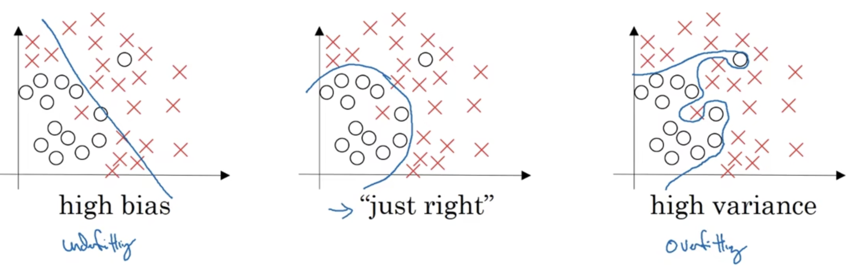
如上图,最左边使用Logistic回归,没有大部分正确分类,属于“欠拟合”的状况;最右边使用比较复杂的神经网络,完整地分出了两个类别,属于”过拟合“的情况(因为部分输入数据是不合理的);中间只有和别数据分类错误,这叫“适度拟合”,是我们比较追求的一种状态。
上图这种只有一个或者两个特征的二维数据中,可以绘制数据,将偏差和方差可视化。但在多维空间数据中,绘制数据和可视化分割边界无法实现。
我们在多维空间通常通过两个个指标,来研究偏差和方差:训练集误差和测试集误差。为了便于研究,假设人眼分辨的错误率为0,这也被称为基本误差或者最优误差;假设训练集和验证集来自同一分布。如果训练集误差为0.01,测试集误差为0.11,这种情况很有可能是我们过度拟合了训练集,称之为高方差,对应于上图最右边的情况;如果训练集误差为0.15,测试集误差为0.16,这种情况很有可能是我们训练数据的时候欠拟合,称之为高偏差,对应于上图最左边的情况;如果训练集误差为0.15,测试集误差为0.3,偏差和方差都比较高,这种情况是因为你的算法模型并不适合这个任务,需要改变模型;如果训练集误差为0.005,测试集误差为0.01,偏差和方差都很低,是分类效果比较好的情况,对应上图中间的情况。
模型评估调优的过程
- 首先,将进行训练之后的模型用于评估训练集的性能,如果误差高,代表欠拟合。那么你要采取的方法可能是增加训练时间或者增大网络结构或者是选择一个新网络,先将偏差降下来,拟合训练数据。(这在基本误差不同的情况下会有所不同)
- 如果模型的训练集性能很高后,可以将其用于评估测试集,如果误差高,代表过拟合。那么你要采取的方法最好是采用更多的训练数据,如果无法获得更多数据,可以通过正则化来减少过拟合,降低方差,有时候也会通过替换网络结构来实现。
正则化
如果你的模型在评估是,由比较高的方差,然而你又不能拿到更多的数据集,那么我们最先想到的办法可能是正则化。
正则化有助于避免数据过度拟合,减少网络误差。
假设我们的目标是找到$w,b$来使得$J(w,b)$达到最小值,且使用逻辑回归的代价函数,那么
$$
J(w,b)=\frac1m\sum^m_{i=1}L(\hat{y}^{(i)},y^{(i)})
$$
我们在该函数中加入正则化
$$
J(w,b)=\frac1m\sum^m_{i=1}L(\hat{y}^{(i)},y^{(i)})+\frac{\lambda}{2m}{\Vert w \Vert_2}^2\
{\Vert w \Vert_2}^2=\sum^{n_x}{j=1}w{j}^2=w^Tw \quad 这被称为L2正则化
$$
同理也会有L正则化
$$
J(w,b)=\frac1m\sum^m_{i=1}L(\hat{y}^{(i)},y^{(i)})+\frac{\lambda}{m}{\Vert w \Vert_1}\
{\Vert w \Vert_1}=\sum^{n_x}_{j=1}\lvert w_j \rvert \quad 这被称为L1正则化
$$
通常我们都会使用L2正则化来实现降低方差的效果。
那么$\lambda$的值我们需要如何确定呢?
我们通常使用验证集或者交叉验证来配置$\lambda$参数,不过首先要考虑训练集之间的权衡,吧参数$w,b$正常值设为较小的值,避免过拟合,不断调整超参数$\lambda$的值来减小方差。
需要特别说明的是在编写代码的时候,python语言中lambda是一个保留字段,所以编程时我们通常使用lambd来代替lambda。
$$
J(W^{[1]},b^{[1]},\dots,W^{[L]},b^{[L]})=\frac1m\sum^n_{i=1}L(\hat{y}^{(i)},y^{(i)})+ \frac{\lambda}{2m}\sum^L_{l=1}{\Vert W^{[l]} \Vert}^2\
{\Vert W^{[l]} \Vert}^2=\sum_{i=1}^{n^{[l]}}\sum_{j=1}^{n^{[l-1]}}(W_{i,j}^{[l]})^2\quad 该矩阵范数被称为是弗罗贝尼乌斯范数\
W的维度是(n^{[l]},n^{[l-1]})
$$
如果$J(W,b)$发生了改变,那么反向传播的$dW^{[l]}$也要发生变化:
在backprop计算出的$dW$的基础上加一个$\frac{\lambda}{m}W^{[l]}$,然后用此更新$W^{[l]}$的值,这样做的结果是的$W^{[l]}$会比没有正则化之前更小。因此L2范数也被称为权重衰减。
正则化如何预防过拟合
如果正则化的参数$\lambda$如果设置的过大,$W^{[l]}$会变得更小,就会导致每层上的部分$w$的权重 会接近0,这相当于将部分隐藏单元给去除了,复杂的神经网络会退化称为一 个很深但是又很简单的网络,导致从过拟合直接变成欠拟合的状态。
一个合适的$\lambda$值能够使模型的性能从过拟合到适度拟合。
$\lambda$越大,得到迭代的$W$就越小,这相当于让部分隐藏单元的影响变小,降低模型的拟合程度,方差减小。
总体来说,正则化的效果其实就是将复杂的网络线性化,如果$\lambda$的取值设置的比较好,能达到适度拟合的效果。
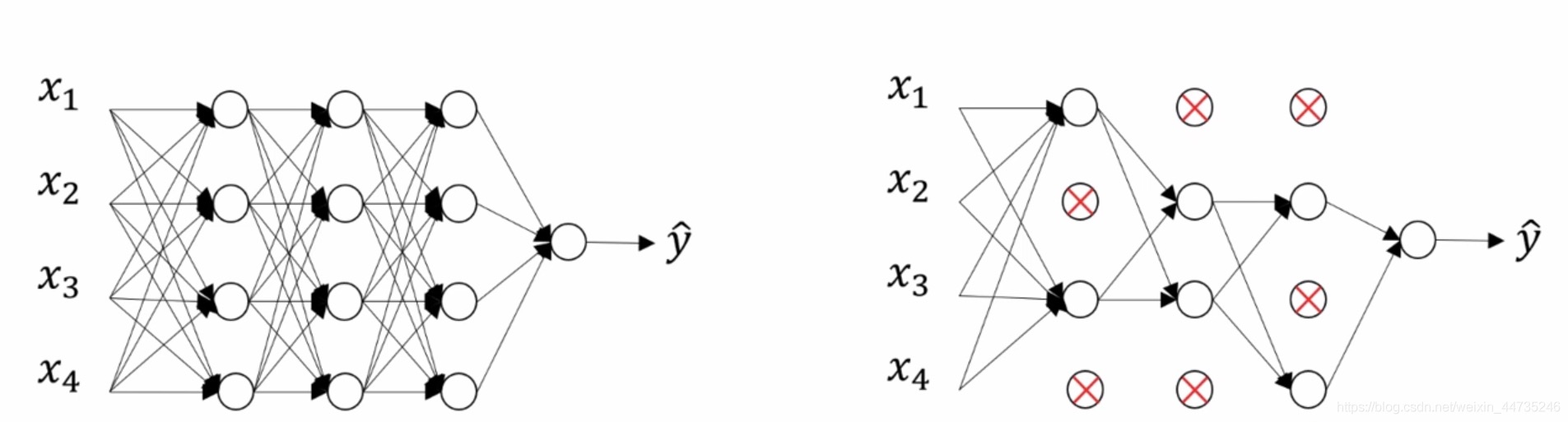
dropout正则化
dropout正则化是指如果一个网络存在过拟合的情况下,可以将所有节点(隐藏单元)设置一个删除概率为0.5,那么保留该隐藏单元的概率keep-prob也为0.5,这个值是可以改变的,然后随机消除一些节点并删除该节点进出的连线,得到一个节点更少,规模更小的网络。如下图所示:
实现Dropout的方法很多,最常用的是inverted dropout。以一个深层神经网络的某一个隐藏层为例来解释怎么进行Dropout正则化。首先假设对于第$l$层,其激活函数为$a^{[l]}$,我们设置的保留概率keep_prob等于0.8,这意味着该隐藏层的所有神经元以0.8的概率得到保留。
可以将inverted dropout方法归纳为四步:
1.根据keep_prob生成和 $a^{[l]}$相同的随机概率矩阵$d^{[l]}$,Dl = np.rndom.randn(Al.shape[0], Al.shape[1])
2.将$d^{[l]}$转化为0-1矩阵, Dl = Dl < keep_prob
3.将$a^{[l]}$和$d^{[l]}$ 中的元素一一对应相乘,$d^{[l]}$为1代表对应的神经元被保留,$d^{[l]}$为0则代表舍弃, Al = np.muiltiply(Al, Dl)
4.为了确保$a^{[l]}$的期望值不变,将$a^{[l]}$除以keep_prob,Al = Al / keep_prob
需要注意的是,在反向传播的时候,也需要像上面一样进行dropout操作,和前向传播关闭相同的神经元。即对于某一层的$da^{[l]}$,应该进行以下计算:
1.dAl = dAl * Dl
2.dAl = dAl / keep_prob
另一点是,Dropout正则化只在训练阶段实施,在测试阶段只需要利用训练好的参数进行正向预测,而不需要进行神经元的随机失活。
三层网络的前向传播dropout示例代码:
 1
 2
 3
 4
 5
 6
 7
 8
 9
10
11
12
13
14
|
keep_prob = 0.8
def foward(X):
    # 3层neural network的前向传播
    A1 = np.maximum(0, np.dot(W1, X) + b1)  # 计算第一层网络的输出
    D1 = (np.random.rand(*A1.shape) < keep_prob)  # 以keep_prob为标准,判断该层结点哪些可以保留
    Z1 = np.multiply(A1, D1)     #dropout
    Z1 /= keep_prob   # 为了期望的一致,除以keep_prob

    A2 = np.maximum(0, np.dot(W2, Z1) + b2)
    D2 = (np.random.rand(*A2.shape) < keep_prob)
    Z2 = np.multiply(A2, D2)
    Z2 /= keep_prob

    out = np.dot(W3, Z2) + b3
|
那么我们如何在不同的层设置不同的keep_prob,我们可以在不太会发生过拟合现象的地方设置keep_prob为1,在容易发生过拟合的地方将keep_prob设置的低一点。
使用drop_out正则化的缺点是不能定义明确的代价函数,那么我们使用的方法一般是先将drop_out关闭,确保该网络的代价函数是递减的,再打开drop_out进行学习。
数据扩容
在我们数据不够的情况下,可以在已有的数据的基础上将数据进行稍作改变来增加数据集。举个例子,一张包含猫咪的图片,我们可以将其扩容为几张:
1.将猫的图片进行水平翻转,得到一张新的图片
2.将猫的图片进行局部放大,并进行裁剪
但是最重要的一点就是经过调整后的图片,必须确保它还是一只猫。
如果输入的是一个数字,我们可以将这些数字进行轻微扭曲,旋转,将其加入数据集。
- Early stopping:一种防止过拟合的方法。
使用该方法可以绘制训练集的误差和验证集的误差,可以用来预防过拟合。
L2正则化和early stopping的对比:
1.L2正则化训练神经网络的时间可能很长。这导致超参数搜索空间更容易分解
2.L2正则化可能许多正则化参数$\lambda$的值,计算代价太高。而early stopping只运行一次梯度下降,你就可以找到W的最大值,中间值,最小值,无需多次迭代。
归一化输入
如图,给定输入数据的散点图:
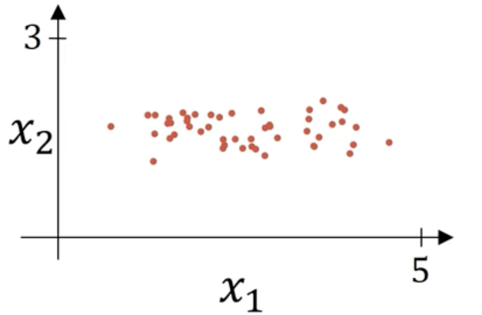
归一化需要两个步骤:
$$
u=\frac1m\sum_{i=1}^mX^{(i)}\
x:=X-u
$$
意思是移动训练集,直至它完成零均值化,结果如下:
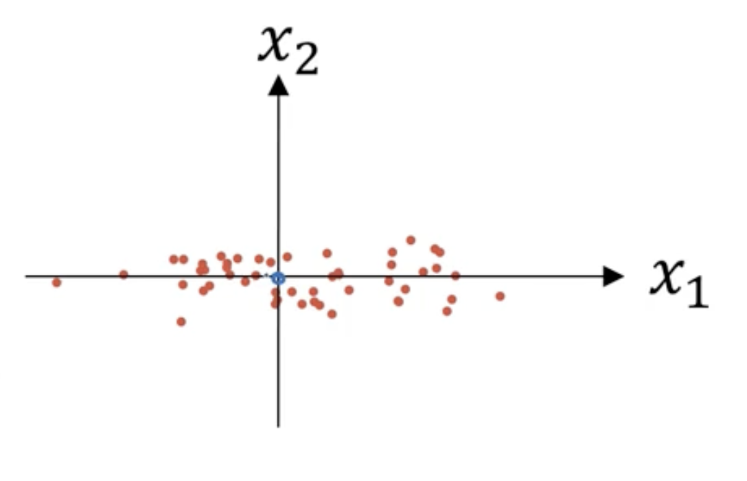
如上图可以看到,特征$x_1$的方差比特征$x_2$大得多。使用如下公式迭代:
$$
\sigma^2=\frac1m\sum_{i=1}^mx^{(i)}**2\
x/=\sigma^2
$$
结果如下:
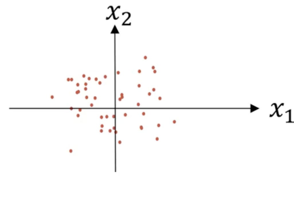
需要注意的是:我们在训练集和验证集或者测试集上需要设置相同的$u$和$\sigma^2$
那么为什么要使用归一化呢?
归一化会使得不同的特征的起始$W$范围较为接近,使得它们的代价函数有如下图的转变:
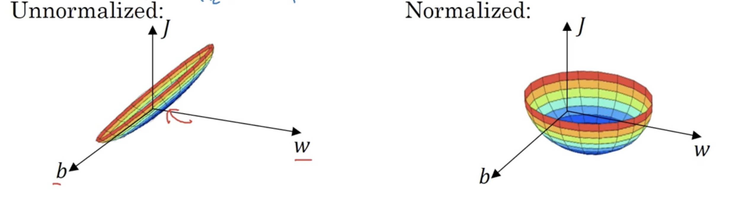
这样可以减少迭代,使得梯度下降法使用更大的步长。
梯度消失和梯度爆炸
在深度神经网络中梯度是不稳定的,可能会变得非常小,也可能会变得非常大,这就是梯度消失和梯度爆炸。
假设$W^{[1]}$比单位矩阵稍微大一点,那么在深度神经网络中,激活函数将会是指数级增长 ;相反,假设$W^{[1]}$比单位矩阵稍微小一些,激活函数会呈现指数级下降的趋势。
那么如何解决如上的问题呢?
一般使用权重初始化来解决:$W^{[l]}=np.random.randn(shape)\times np.sqrt(\frac{1}{n^{[l-1]}})$,其中$shape$代表该层$W$矩阵的维度,$n^{[l-1]}$代表上一层。如果激活函数使用了ReLU激活函数,$\frac{1}{n^{[l-1]}}$可以变成$\frac{2}{n^{[l-1]}}$效果更好;如果使用tanh激活函数,使用$\frac{1}{n^{[l-1]}}$;有时候也会看到使用$np.sqrt(\frac{1}{n^{[l-1]}+n^{[l]}})$。
梯度检验
关于梯度的数值逼近,一般使用双边误差公式,即
$$
f^{’}(\theta)=\frac{f(\theta+\epsilon)-f(\theta-\epsilon)}{2\epsilon}
$$
我们通常会通过梯度检验来验证backprop过程的正确实施:
首先,我们需要将$W^{[1]},b^{[1]},\dots,W^{[L]},b^{[L]}$重新组合成为一个大的向量$\theta$;同样的,在反向传播的过程也需要将$dW^{[1]},db^{[1]},\dots,dW^{[L]},db^{[L]}$重新组合成为一个大的向量$d\theta$。
$$
J(\theta)=J(\theta_1,\theta_2,\dots)
$$
然后对于每个$i$:
$$
{d\theta_{approx}}^{[i]}=\lim_{\epsilon\rightarrow0}\frac{J(\theta_1,\theta_2,\dots,\theta_{i+\epsilon},\dots)-J(\theta_1,\theta_2,\dots,\theta_{i-\epsilon},\dots)}{2\epsilon}\approx d\theta^{[i]}=\frac{\partial J}{\partial \theta_i}
$$
做完计算之后,需要做的就是验证是否:
$$
d\theta_{approx}\approx d\theta
$$
如果上述两个量差值的二范数在$10^{-7}$量级,这代表导数逼近很有可能是正确的;如果在$10^{-5}$,就需要担心是否是正确的;如果在$10^{-3}$,那说明你的梯度下降传播程序出现了bug。
注意事项:
1.梯度检验是非常耗费时间的,在训练的时候不使用梯度检验,只有在debug的时候使用。
2.如果算法的梯度检验失败,要检查每一项,找出bug。
3.如果代价函数包含了正则项$\frac{\lambda}{2m}{\Vert w \Vert_2}^2$,那么$d\theta_{approx}$也需要多加一个正则项。
4.梯度检验和dropout正则化不能同时使用。所以在梯度检验的时候,需要先关闭dropout正则化。
作业四
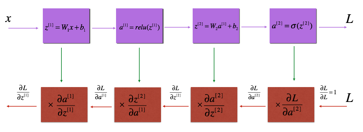
其工作原理如下:
前向传播和后向传播示例代码:
 1
 2
 3
 4
 5
 6
 7
 8
 9
10
11
12
13
14
15
16
17
18
19
20
21
22
23
24
25
26
27
28
29
30
31
32
33
34
35
36
37
38
39
40
41
42
43
44
45
46
47
48
49
50
51
52
53
54
55
56
57
58
59
60
61
62
63
64
65
66
67
68
69
70
71
72
73
74
75
76
77
78
79
80
81
82
83
84
|
import numpy as np
from gc_utils import sigmoid, relu, dictionary_to_vector, vector_to_dictionary, gradients_to_vector

#-------------------------------------------------
def forward_propagation_n(X, Y, parameters):
    """
    Implements the forward propagation (and computes the cost) presented in Figure 3.

    Arguments:
    X -- training set for m examples
    Y -- labels for m examples
    parameters -- python dictionary containing your parameters "W1", "b1", "W2", "b2", "W3", "b3":
                    W1 -- weight matrix of shape (5, 4)
                    b1 -- bias vector of shape (5, 1)
                    W2 -- weight matrix of shape (3, 5)
                    b2 -- bias vector of shape (3, 1)
                    W3 -- weight matrix of shape (1, 3)
                    b3 -- bias vector of shape (1, 1)

    Returns:
    cost -- the cost function (logistic cost for one example)
    """

    # retrieve parameters
    m = X.shape[1]
    W1 = parameters["W1"]
    b1 = parameters["b1"]
    W2 = parameters["W2"]
    b2 = parameters["b2"]
    W3 = parameters["W3"]
    b3 = parameters["b3"]

    # LINEAR -> RELU -> LINEAR -> RELU -> LINEAR -> SIGMOID
    Z1 = np.dot(W1, X) + b1
    A1 = relu(Z1)
    Z2 = np.dot(W2, A1) + b2
    A2 = relu(Z2)
    Z3 = np.dot(W3, A2) + b3
    A3 = sigmoid(Z3)

    # Cost
    logprobs = np.multiply(-np.log(A3),Y) + np.multiply(-np.log(1 - A3), 1 - Y)
    cost = 1./m * np.sum(logprobs)

    cache = (Z1, A1, W1, b1, Z2, A2, W2, b2, Z3, A3, W3, b3)

    return cost, cache

#-------------------------------------------------
def backward_propagation_n(X, Y, cache):
    """
    Implement the backward propagation presented in figure 2.

    Arguments:
    X -- input datapoint, of shape (input size, 1)
    Y -- true "label"
    cache -- cache output from forward_propagation_n()

    Returns:
    gradients -- A dictionary with the gradients of the cost with respect to each parameter, activation and pre-activation variables.
    """

    m = X.shape[1]
    (Z1, A1, W1, b1, Z2, A2, W2, b2, Z3, A3, W3, b3) = cache

    dZ3 = A3 - Y
    dW3 = 1./m * np.dot(dZ3, A2.T)
    db3 = 1./m * np.sum(dZ3, axis=1, keepdims = True)

    dA2 = np.dot(W3.T, dZ3)
    dZ2 = np.multiply(dA2, np.int64(A2 > 0))
    dW2 = 1./m * np.dot(dZ2, A1.T) * 2
    db2 = 1./m * np.sum(dZ2, axis=1, keepdims = True)

    dA1 = np.dot(W2.T, dZ2)
    dZ1 = np.multiply(dA1, np.int64(A1 > 0))
    dW1 = 1./m * np.dot(dZ1, X.T)
    db1 = 4./m * np.sum(dZ1, axis=1, keepdims = True)

    gradients = {"dZ3": dZ3, "dW3": dW3, "db3": db3,
                 "dA2": dA2, "dZ2": dZ2, "dW2": dW2, "db2": db2,
                 "dA1": dA1, "dZ1": dZ1, "dW1": dW1, "db1": db1}

    return gradients
|
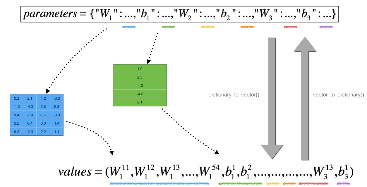
接下去就需要进行梯度检验了!其中涉及的字典转vector的原理图如下:
梯度检验的代码如下:
 1
 2
 3
 4
 5
 6
 7
 8
 9
10
11
12
13
14
15
16
17
18
19
20
21
22
23
24
25
26
27
28
29
30
31
32
33
34
35
36
37
38
39
40
41
42
43
44
45
46
47
48
49
50
51
52
53
54
55
56
57
58
59
60
61
|
def gradient_check_n(parameters, gradients, X, Y, epsilon = 1e-7):
    """
    Checks if backward_propagation_n computes correctly the gradient of the cost output by forward_propagation_n

    Arguments:
    parameters -- python dictionary containing your parameters "W1", "b1", "W2", "b2", "W3", "b3":
    grad -- output of backward_propagation_n, contains gradients of the cost with respect to the parameters.
    x -- input datapoint, of shape (input size, 1)
    y -- true "label"
    epsilon -- tiny shift to the input to compute approximated gradient with formula(1)

    Returns:
    difference -- difference (2) between the approximated gradient and the backward propagation gradient
    """

    # Set-up variables
    parameters_values, _ = dictionary_to_vector(parameters)
    grad = gradients_to_vector(gradients)
    num_parameters = parameters_values.shape[0]
    J_plus = np.zeros((num_parameters, 1))
    J_minus = np.zeros((num_parameters, 1))
    gradapprox = np.zeros((num_parameters, 1))

    # Compute gradapprox
    for i in range(num_parameters):

        # Compute J_plus[i]. Inputs: "parameters_values, epsilon". Output = "J_plus[i]".
        # "_" is used because the function you have to outputs two parameters but we only care about the first one
        ### START CODE HERE ### (approx. 3 lines)
        epsilon = 0.01
        thetaplus = np.copy(parameters_values)                                      # Step 1
        thetaplus[i][0] = thetaplus[i][0] + epsilon                                # Step 2
        J_plus[i], _ = forward_propagation_n(X, Y, vector_to_dictionary(thetaplus))                                   # Step 3
        ### END CODE HERE ###

        # Compute J_minus[i]. Inputs: "parameters_values, epsilon". Output = "J_minus[i]".
        ### START CODE HERE ### (approx. 3 lines)
        thetaminus = np.copy(parameters_values)                                     # Step 1
        thetaminus[i][0] = thetaminus[i][0] - epsilon                               # Step 2
        J_minus[i], _ = forward_propagation_n(X, Y, vector_to_dictionary(thetaminus))                                  # Step 3
        ### END CODE HERE ###

        # Compute gradapprox[i]
        ### START CODE HERE ### (approx. 1 line)
        gradapprox[i] = (J_plus[i] - J_minus[i]) / (2*epsilon)
        ### END CODE HERE ###

    # Compare gradapprox to backward propagation gradients by computing difference.
    ### START CODE HERE ### (approx. 1 line)
    # np.linalg.norm()的作用是求二范数
    numerator = np.linalg.norm(grad)                                           # Step 1'
    denominator = np.linalg.norm(gradapprox)                                         # Step 2'
    difference = np.linalg.norm(grad - gradapprox) / (numerator + denominator)                                          # Step 3'
    ### END CODE HERE ###

    if difference > 1e-7:
        print ("\033[93m" + "There is a mistake in the backward propagation! difference = " + str(difference) + "\033[0m")
    else:
        print ("\033[92m" + "Your backward propagation works perfectly fine! difference = " + str(difference) + "\033[0m")

    return difference
|
下列代码会通过三种初始化的方式进行对比:
1.将W和b都设置为0向量
2.随机设置W和b
3.在随机设置的基础上进行权重初始化
代码如下:
加载初始数据:
 1
 2
 3
 4
 5
 6
 7
 8
 9
10
11
12
13
14
|
import numpy as np
import matplotlib.pyplot as plt
import sklearn
import sklearn.datasets
from init_utils import sigmoid, relu, compute_loss, forward_propagation, backward_propagation
from init_utils import update_parameters, predict, load_dataset, plot_decision_boundary, predict_dec
%matplotlib inline
plt.rcParams['figure.figsize'] = (7.0, 4.0) # set default size of plots
plt.rcParams['image.interpolation'] = 'nearest'
plt.rcParams['image.cmap'] = 'gray'
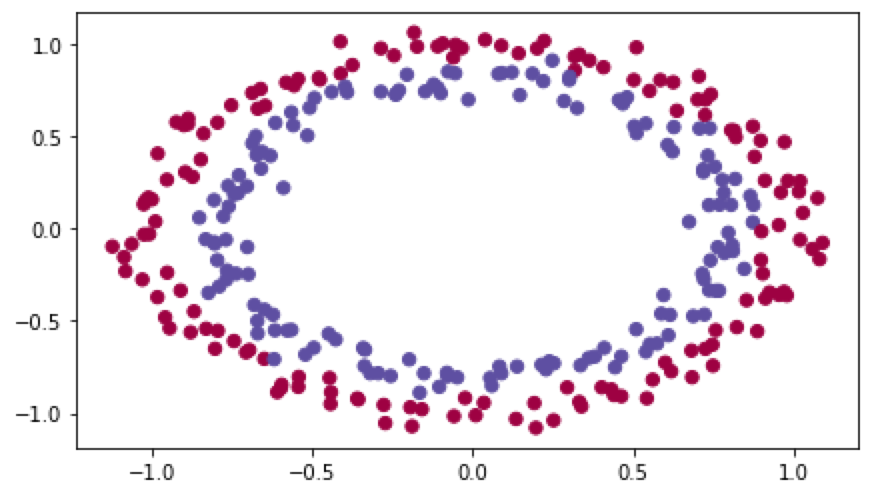
# load image dataset: blue/red dots in circles
train_X, train_Y, test_X, test_Y = load_dataset()
|
结果如下:
初始化模型:
 1
 2
 3
 4
 5
 6
 7
 8
 9
10
11
12
13
14
15
16
17
18
19
20
21
22
23
24
25
26
27
28
29
30
31
32
33
34
35
36
37
38
39
40
41
42
43
44
45
46
47
48
49
50
51
52
53
54
55
56
57
58
|
def model(X, Y, learning_rate = 0.01, num_iterations = 15000, print_cost = True, initialization = "he"):
    """
    Implements a three-layer neural network: LINEAR->RELU->LINEAR->RELU->LINEAR->SIGMOID.

    Arguments:
    X -- input data, of shape (2, number of examples)
    Y -- true "label" vector (containing 0 for red dots; 1 for blue dots), of shape (1, number of examples)
    learning_rate -- learning rate for gradient descent
    num_iterations -- number of iterations to run gradient descent
    print_cost -- if True, print the cost every 1000 iterations
    initialization -- flag to choose which initialization to use ("zeros","random" or "he")

    Returns:
    parameters -- parameters learnt by the model
    """

    grads = {}
    costs = [] # to keep track of the loss
    m = X.shape[1] # number of examples
    layers_dims = [X.shape[0], 10, 5, 1]

    # Initialize parameters dictionary.
    if initialization == "zeros":
        parameters = initialize_parameters_zeros(layers_dims)
    elif initialization == "random":
        parameters = initialize_parameters_random(layers_dims)
    elif initialization == "he":
        parameters = initialize_parameters_he(layers_dims)

    # Loop (gradient descent)

    for i in range(0, num_iterations):

        # Forward propagation: LINEAR -> RELU -> LINEAR -> RELU -> LINEAR -> SIGMOID.
        a3, cache = forward_propagation(X, parameters)

        # Loss
        cost = compute_loss(a3, Y)

        # Backward propagation.
        grads = backward_propagation(X, Y, cache)

        # Update parameters.
        parameters = update_parameters(parameters, grads, learning_rate)

        # Print the loss every 1000 iterations
        if print_cost and i % 1000 == 0:
            print("Cost after iteration {}: {}".format(i, cost))
            costs.append(cost)

    # plot the loss
    plt.plot(costs)
    plt.ylabel('cost')
    plt.xlabel('iterations (per hundreds)')
    plt.title("Learning rate =" + str(learning_rate))
    plt.show()

    return parameters
|
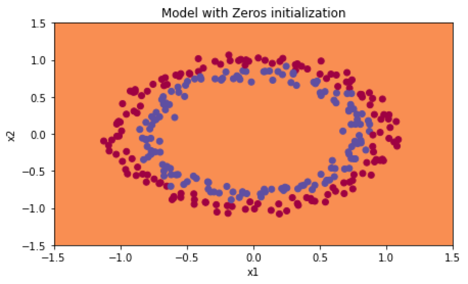
W为0向量初始化:
 1
 2
 3
 4
 5
 6
 7
 8
 9
10
11
12
13
14
15
16
17
18
19
20
21
22
23
24
25
26
27
28
29
30
31
32
33
34
35
36
37
38
39
40
41
42
43
44
45
46
47
48
49
50
51
52
53
54
55
56
57
58
59
|
def initialize_parameters_zeros(layers_dims):
    """
    Arguments:
    layer_dims -- python array (list) containing the size of each layer.

    Returns:
    parameters -- python dictionary containing your parameters "W1", "b1", ..., "WL", "bL":
                    W1 -- weight matrix of shape (layers_dims[1], layers_dims[0])
                    b1 -- bias vector of shape (layers_dims[1], 1)
                    ...
                    WL -- weight matrix of shape (layers_dims[L], layers_dims[L-1])
                    bL -- bias vector of shape (layers_dims[L], 1)
    """

    parameters = {}
    L = len(layers_dims)            # number of layers in the network

    for i in range(1, L):
        ### START CODE HERE ### (≈ 2 lines of code)
        parameters['W' + str(i)] = np.zeros((layers_dims[i], layers_dims[i - 1]))
        parameters['b' + str(i)] = np.zeros((layers_dims[i], 1))
        ### END CODE HERE ###
    return parameters

#---------------------------------------------
parameters = initialize_parameters_zeros([3,2,1])
parameters = model(train_X, train_Y, initialization = "zeros")
print ("On the train set:")
predictions_train = predict(train_X, train_Y, parameters)
print ("On the test set:")
predictions_test = predict(test_X, test_Y, parameters)

#---------------------------------------------
# 画图
def plot_decision_boundary(model, X, y):
    #import pdb;pdb.set_trace()
    # Set min and max values and give it some padding
    x_min, x_max = X[0, :].min() - 1, X[0, :].max() + 1
    y_min, y_max = X[1, :].min() - 1, X[1, :].max() + 1
    h = 0.01
    # Generate a grid of points with distance h between them
    xx, yy = np.meshgrid(np.arange(x_min, x_max, h), np.arange(y_min, y_max, h))
    # Predict the function value for the whole grid
    Z = model(np.c_[xx.ravel(), yy.ravel()])
    Z = Z.reshape(xx.shape)
    # Plot the contour and training examples
    plt.contourf(xx, yy, Z, cmap=plt.cm.Spectral)
    plt.ylabel('x2')
    plt.xlabel('x1')
    y = y.reshape(X[0,:].shape)#must reshape,otherwise confliction with dimensions
    plt.scatter(X[0, :], X[1, :], c=y, cmap=plt.cm.Spectral)
    plt.show()

#---------------------------------------------
plt.title("Model with Zeros initialization")
axes = plt.gca()
axes.set_xlim([-1.5,1.5])
axes.set_ylim([-1.5,1.5])
plot_decision_boundary(lambda x: predict_dec(parameters, x.T), train_X, train_Y)
|
分类结果如下:
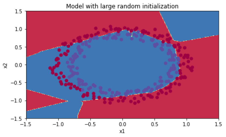
W为随机向量初始化:
 1
 2
 3
 4
 5
 6
 7
 8
 9
10
11
12
13
14
15
16
17
18
19
20
21
22
23
24
25
26
27
28
29
30
31
32
33
34
35
36
37
38
39
40
41
|
def initialize_parameters_random(layers_dims):
    """
    Arguments:
    layer_dims -- python array (list) containing the size of each layer.

    Returns:
    parameters -- python dictionary containing your parameters "W1", "b1", ..., "WL", "bL":
                    W1 -- weight matrix of shape (layers_dims[1], layers_dims[0])
                    b1 -- bias vector of shape (layers_dims[1], 1)
                    ...
                    WL -- weight matrix of shape (layers_dims[L], layers_dims[L-1])
                    bL -- bias vector of shape (layers_dims[L], 1)
    """

    np.random.seed(3)               # This seed makes sure your "random" numbers will be the as ours
    parameters = {}
    L = len(layers_dims)            # integer representing the number of layers

    for i in range(1, L):
        ### START CODE HERE ### (≈ 2 lines of code)
        parameters['W' + str(i)] = np.random.randn(layers_dims[i], layers_dims[i - 1]) * 10
        parameters['b' + str(i)] = np.zeros((layers_dims[i], 1))
        ### END CODE HERE ###

    return parameters

#---------------------------------------------
parameters = initialize_parameters_random([3, 2, 1])
parameters = model(train_X, train_Y, initialization = "random")
print ("On the train set:")
predictions_train = predict(train_X, train_Y, parameters)
print ("On the test set:")
predictions_test = predict(test_X, test_Y, parameters)

#---------------------------------------------
# 画图
plt.title("Model with large random initialization")
axes = plt.gca()
axes.set_xlim([-1.5,1.5])
axes.set_ylim([-1.5,1.5])
plot_decision_boundary(lambda x: predict_dec(parameters, x.T), train_X, train_Y)
|
分类结果如下:
W为权重初始化后的结果,因为这里使用的ReLU激活函数,W在初始化后需要变为$W^{[l]}=np.random.randn(shape)\times np.sqrt(\frac{2}{n^{[l-1]}})$:
 1
 2
 3
 4
 5
 6
 7
 8
 9
10
11
12
13
14
15
16
17
18
19
20
21
22
23
24
25
26
27
28
29
30
31
32
33
34
35
36
37
38
39
40
41
|
def initialize_parameters_he(layers_dims):
    """
    Arguments:
    layer_dims -- python array (list) containing the size of each layer.

    Returns:
    parameters -- python dictionary containing your parameters "W1", "b1", ..., "WL", "bL":
                    W1 -- weight matrix of shape (layers_dims[1], layers_dims[0])
                    b1 -- bias vector of shape (layers_dims[1], 1)
                    ...
                    WL -- weight matrix of shape (layers_dims[L], layers_dims[L-1])
                    bL -- bias vector of shape (layers_dims[L], 1)
    """

    np.random.seed(3)
    parameters = {}
    L = len(layers_dims) - 1 # integer representing the number of layers

    for i in range(1, L + 1):
        ### START CODE HERE ### (≈ 2 lines of code)
        parameters['W' + str(i)] = np.random.randn(layers_dims[i],layers_dims[i - 1]) * np.sqrt(2.0 / layers_dims[i - 1])
        parameters['b' + str(i)] = np.zeros((layers_dims[i], 1))
        ### END CODE HERE ###

    return parameters

#---------------------------------------------
parameters = initialize_parameters_he([2, 4, 1])
parameters = model(train_X, train_Y, initialization = "he")
print ("On the train set:")
predictions_train = predict(train_X, train_Y, parameters)
print ("On the test set:")
predictions_test = predict(test_X, test_Y, parameters)

#---------------------------------------------
# 画图
plt.title("Model with He initialization")
axes = plt.gca()
axes.set_xlim([-1.5,1.5])
axes.set_ylim([-1.5,1.5])
plot_decision_boundary(lambda x: predict_dec(parameters, x.T), train_X, train_Y)
|
分类结果如下:
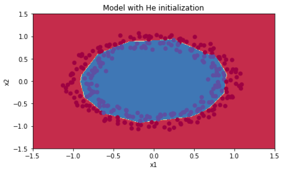
可以看到第三种的分类效果最好!
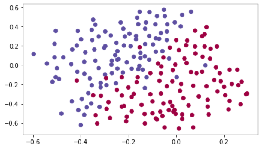
加载数据:
 1
 2
 3
 4
 5
 6
 7
 8
 9
10
11
12
13
14
15
|
import numpy as np
import matplotlib.pyplot as plt
from reg_utils import sigmoid, relu, plot_decision_boundary, initialize_parameters, load_2D_dataset, predict_dec
from reg_utils import compute_cost, predict, forward_propagation, backward_propagation, update_parameters
import sklearn
import sklearn.datasets
import scipy.io
from testCases import *

%matplotlib inline
plt.rcParams['figure.figsize'] = (7.0, 4.0) # set default size of plots
plt.rcParams['image.interpolation'] = 'nearest'
plt.rcParams['image.cmap'] = 'gray'

train_X, train_Y, test_X, test_Y = load_2D_dataset()
|
数据的分布如下图:
使用无正则化模型,进行梯度下降:
 1
 2
 3
 4
 5
 6
 7
 8
 9
10
11
12
13
14
15
16
17
18
19
20
21
22
23
24
25
26
27
28
29
30
31
32
33
34
35
36
37
38
39
40
41
42
43
44
45
46
47
48
49
50
51
52
53
54
55
56
57
58
59
60
61
62
63
64
65
66
67
68
69
70
71
72
73
74
75
76
77
78
79
80
81
82
83
|
# 这里其实已经包含了L2正则化和dropout正则化的情况,只默认情况下的参数不使用正则化
def model(X, Y, learning_rate = 0.3, num_iterations = 30000, print_cost = True, lambd = 0, keep_prob = 1):
"""
Implements a three-layer neural network: LINEAR->RELU->LINEAR->RELU->LINEAR->SIGMOID.
Arguments:
X -- input data, of shape (input size, number of examples)
Y -- true "label" vector (1 for blue dot / 0 for red dot), of shape (output size, number of examples)
learning_rate -- learning rate of the optimization
num_iterations -- number of iterations of the optimization loop
print_cost -- If True, print the cost every 10000 iterations
lambd -- regularization hyperparameter, scalar
keep_prob - probability of keeping a neuron active during drop-out, scalar.
Returns:
parameters -- parameters learned by the model. They can then be used to predict.
"""
grads = {}
costs = [] # to keep track of the cost
m = X.shape[1] # number of examples
layers_dims = [X.shape[0], 20, 3, 1] # 网络结构为三层网络结构,分别有20,3,1个节点
# Initialize parameters dictionary.
parameters = initialize_parameters(layers_dims)
# Loop (gradient descent)
for i in range(0, num_iterations):
# Forward propagation: LINEAR -> RELU -> LINEAR -> RELU -> LINEAR -> SIGMOID.
if keep_prob == 1:
a3, cache = forward_propagation(X, parameters)
elif keep_prob < 1:
a3, cache = forward_propagation_with_dropout(X, parameters, keep_prob)
# Cost function
if lambd == 0:
cost = compute_cost(a3, Y)
else:
cost = compute_cost_with_regularization(a3, Y, parameters, lambd)
# Backward propagation.
assert(lambd==0 or keep_prob==1) # it is possible to use both L2 regularization and dropout,
# but this assignment will only explore one at a time
if lambd == 0 and keep_prob == 1:
grads = backward_propagation(X, Y, cache)
elif lambd != 0:
grads = backward_propagation_with_regularization(X, Y, cache, lambd)
elif keep_prob < 1:
grads = backward_propagation_with_dropout(X, Y, cache, keep_prob)
# Update parameters.
parameters = update_parameters(parameters, grads, learning_rate)
# Print the loss every 10000 iterations
if print_cost and i % 10000 == 0:
print("Cost after iteration {}: {}".format(i, cost))
if print_cost and i % 1000 == 0:
costs.append(cost)
# plot the cost
plt.plot(costs)
plt.ylabel('cost')
plt.xlabel('iterations (x1,000)')
plt.title("Learning rate =" + str(learning_rate))
plt.show()
return parameters
#----------------------------------------------------
parameters = model(train_X, train_Y)
print ("On the training set:")
predictions_train = predict(train_X, train_Y, parameters)
print ("On the test set:")
predictions_test = predict(test_X, test_Y, parameters)
# 画图
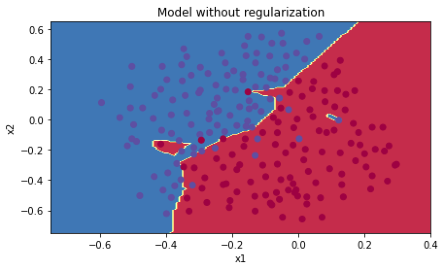
plt.title("Model without regularization")
axes = plt.gca()
axes.set_xlim([-0.75,0.40])
axes.set_ylim([-0.75,0.65])
plot_decision_boundary(lambda x: predict_dec(parameters, x.T), train_X, train_Y)
|
训练集准确率为0.948,测试集准确率为0.915。分类图如下:
使用L2正则化,前向传播公式变化如下:
$$J = -\frac{1}{m} \sum\limits_{i = 1}^{m} \large{(}\small y^{(i)}\log\left(a^{L}\right) + (1-y^{(i)})\log\left(1- a^{L}\right) \large{)} \tag{1}$$
To:
$$J_{regularized} = \small \underbrace{-\frac{1}{m} \sum\limits_{i = 1}^{m} \large{(}\small y^{(i)}\log\left(a^{L}\right) + (1-y^{(i)})\log\left(1- a^{L}\right) \large{)} }\text{cross-entropy cost} + \underbrace{\frac{1}{m} \frac{\lambda}{2} \sum\limits_l\sum\limits_k\sum\limits_j W{k,j}^{[l]2} }_\text{L2 regularization cost} \tag{2}$$
在编程的时候,需要使用np.sum(np.square(W^[l])),然后将所有项加起来,乘上$\frac{\lambda}{2m}$
后向传播时,在backprop计算出的$dW$的基础上加一个$\frac{\lambda}{m}W^{[l]}$,然后用此更新$W^{[l]}$的值。
 1
 2
 3
 4
 5
 6
 7
 8
 9
10
11
12
13
14
15
16
17
18
19
20
21
22
23
24
25
26
27
28
29
30
31
32
33
34
35
36
37
38
39
40
41
42
43
44
45
46
47
48
49
50
51
52
53
54
55
56
57
58
59
60
61
62
63
64
65
66
67
68
69
70
71
72
73
74
75
76
77
78
79
80
81
82
83
84
85
86
87
|
# 前向传播
def compute_cost_with_regularization(A3, Y, parameters, lambd):
"""
Implement the cost function with L2 regularization. See formula (2) above.
Arguments:
A3 -- post-activation, output of forward propagation, of shape (output size, number of examples)
Y -- "true" labels vector, of shape (output size, number of examples)
parameters -- python dictionary containing parameters of the model
Returns:
cost - value of the regularized loss function (formula (2))
"""
m = Y.shape[1]
W1 = parameters["W1"]
W2 = parameters["W2"]
W3 = parameters["W3"]
cross_entropy_cost = compute_cost(A3, Y) # This gives you the cross-entropy part of the cost
### START CODE HERE ### (approx. 1 line)
L2_regularization_cost = lambd * (np.sum(np.square(W1)) + np.sum(np.square(W2)) + np.sum(np.square(W3))) / (2*m)
### END CODER HERE ###
cost = cross_entropy_cost + L2_regularization_cost
return cost
#----------------------------------------------------
# 后向传播
def backward_propagation_with_regularization(X, Y, cache, lambd):
"""
Implements the backward propagation of our baseline model to which we added an L2 regularization.
Arguments:
X -- input dataset, of shape (input size, number of examples)
Y -- "true" labels vector, of shape (output size, number of examples)
cache -- cache output from forward_propagation()
lambd -- regularization hyperparameter, scalar
Returns:
gradients -- A dictionary with the gradients with respect to each parameter, activation and pre-activation variables
"""
m = X.shape[1]
(Z1, A1, W1, b1, Z2, A2, W2, b2, Z3, A3, W3, b3) = cache
dZ3 = A3 - Y
### START CODE HERE ### (approx. 1 line)
dW3 = 1./m * np.dot(dZ3, A2.T) + lambd * W3 / m
### END CODE HERE ###
db3 = 1./m * np.sum(dZ3, axis=1, keepdims = True)
dA2 = np.dot(W3.T, dZ3)
dZ2 = np.multiply(dA2, np.int64(A2 > 0))
### START CODE HERE ### (approx. 1 line)
dW2 = 1./m * np.dot(dZ2, A1.T) + lambd * W2 / m
### END CODE HERE ###
db2 = 1./m * np.sum(dZ2, axis=1, keepdims = True)
dA1 = np.dot(W2.T, dZ2)
dZ1 = np.multiply(dA1, np.int64(A1 > 0))
### START CODE HERE ### (approx. 1 line)
dW1 = 1./m * np.dot(dZ1, X.T) + lambd * W1 / m
### END CODE HERE ###
db1 = 1./m * np.sum(dZ1, axis=1, keepdims = True)
gradients = {"dZ3": dZ3, "dW3": dW3, "db3": db3,"dA2": dA2,
"dZ2": dZ2, "dW2": dW2, "db2": db2, "dA1": dA1,
"dZ1": dZ1, "dW1": dW1, "db1": db1}
return gradients
#----------------------------------------------------
# 使用L2正则化进行梯度下降
parameters = model(train_X, train_Y, lambd = 0.7)
print ("On the train set:")
predictions_train = predict(train_X, train_Y, parameters)
print ("On the test set:")
predictions_test = predict(test_X, test_Y, parameters)
# 画图
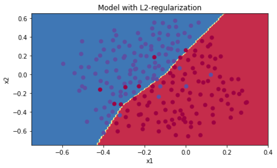
plt.title("Model with L2-regularization")
axes = plt.gca()
axes.set_xlim([-0.75,0.40])
axes.set_ylim([-0.75,0.65])
plot_decision_boundary(lambda x: predict_dec(parameters, x.T), train_X, train_Y)
|
使用L2正则化,训练集的准确率为0.938,测试集为0.93,分类图如下:
使用dropout正则化,在前向传播的时候分为4步:
1.根据keep_prob生成和 $a^{[l]}$相同的随机概率矩阵$d^{[l]}$,Dl = np.rndom.randn(Al.shape[0], Al.shape[1])
2.将$d^{[l]}$转化为0-1矩阵, Dl = Dl < keep_prob
3.将$a^{[l]}$和$d^{[l]}$ 中的元素一一对应相乘,$d^{[l]}$为1代表对应的神经元被保留,$d^{[l]}$为0则代表舍弃, Al = np.muiltiply(Al, Dl)
4.为了确保$a^{[l]}$的期望值不变,将$a^{[l]}$除以keep_prob,Al = Al / keep_prob
后向传播也做修改,即对于某一层的$da^{[l]}$,应该进行以下计算:
1.dAl = dAl * Dl
2.dAl = dAl / keep_prob
代码如下:
  1
  2
  3
  4
  5
  6
  7
  8
  9
 10
 11
 12
 13
 14
 15
 16
 17
 18
 19
 20
 21
 22
 23
 24
 25
 26
 27
 28
 29
 30
 31
 32
 33
 34
 35
 36
 37
 38
 39
 40
 41
 42
 43
 44
 45
 46
 47
 48
 49
 50
 51
 52
 53
 54
 55
 56
 57
 58
 59
 60
 61
 62
 63
 64
 65
 66
 67
 68
 69
 70
 71
 72
 73
 74
 75
 76
 77
 78
 79
 80
 81
 82
 83
 84
 85
 86
 87
 88
 89
 90
 91
 92
 93
 94
 95
 96
 97
 98
 99
100
101
102
103
104
105
106
107
108
109
110
111
112
113
114
115
116
|
# 前向传播
def forward_propagation_with_dropout(X, parameters, keep_prob = 0.5):
"""
Implements the forward propagation: LINEAR -> RELU + DROPOUT -> LINEAR -> RELU + DROPOUT -> LINEAR -> SIGMOID.
Arguments:
X -- input dataset, of shape (2, number of examples)
parameters -- python dictionary containing your parameters "W1", "b1", "W2", "b2", "W3", "b3":
W1 -- weight matrix of shape (20, 2)
b1 -- bias vector of shape (20, 1)
W2 -- weight matrix of shape (3, 20)
b2 -- bias vector of shape (3, 1)
W3 -- weight matrix of shape (1, 3)
b3 -- bias vector of shape (1, 1)
keep_prob - probability of keeping a neuron active during drop-out, scalar
Returns:
A3 -- last activation value, output of the forward propagation, of shape (1,1)
cache -- tuple, information stored for computing the backward propagation
"""
np.random.seed(1)
# retrieve parameters
W1 = parameters["W1"]
b1 = parameters["b1"]
W2 = parameters["W2"]
b2 = parameters["b2"]
W3 = parameters["W3"]
b3 = parameters["b3"]
# LINEAR -> RELU -> LINEAR -> RELU -> LINEAR -> SIGMOID
Z1 = np.dot(W1, X) + b1
A1 = relu(Z1)
### START CODE HERE ### (approx. 4 lines) # Steps 1-4 below correspond to the Steps 1-4 described above.
D1 = np.random.rand(*A1.shape) # Step 1: initialize matrix D1 = np.random.rand(..., ...)
D1 = D1 < keep_prob # Step 2: convert entries of D1 to 0 or 1 (using keep_prob as the threshold)
A1 = np.multiply(A1, D1) # Step 3: shut down some neurons of A1
A1 = A1 / keep_prob # Step 4: scale the value of neurons that haven't been shut down
### END CODE HERE ###
Z2 = np.dot(W2, A1) + b2
A2 = relu(Z2)
### START CODE HERE ### (approx. 4 lines)
D2 = np.random.rand(*A2.shape) # Step 1: initialize matrix D2 = np.random.rand(..., ...)
D2 = D2 < keep_prob # Step 2: convert entries of D2 to 0 or 1 (using keep_prob as the threshold)
A2 = np.multiply(A2, D2) # Step 3: shut down some neurons of A2
A2 = A2 / keep_prob # Step 4: scale the value of neurons that haven't been shut down
### END CODE HERE ###
Z3 = np.dot(W3, A2) + b3
A3 = sigmoid(Z3)
cache = (Z1, D1, A1, W1, b1, Z2, D2, A2, W2, b2, Z3, A3, W3, b3)
return A3, cache
#----------------------------------------------
# 后向传播
def backward_propagation_with_dropout(X, Y, cache, keep_prob):
"""
Implements the backward propagation of our baseline model to which we added dropout.
Arguments:
X -- input dataset, of shape (2, number of examples)
Y -- "true" labels vector, of shape (output size, number of examples)
cache -- cache output from forward_propagation_with_dropout()
keep_prob - probability of keeping a neuron active during drop-out, scalar
Returns:
gradients -- A dictionary with the gradients with respect to each parameter, activation and pre-activation variables
"""
m = X.shape[1]
(Z1, D1, A1, W1, b1, Z2, D2, A2, W2, b2, Z3, A3, W3, b3) = cache
dZ3 = A3 - Y
dW3 = 1./m * np.dot(dZ3, A2.T)
db3 = 1./m * np.sum(dZ3, axis=1, keepdims = True)
dA2 = np.dot(W3.T, dZ3)
### START CODE HERE ### (≈ 2 lines of code)
dA2 = dA2 * D2 # Step 1: Apply mask D2 to shut down the same neurons as during the forward propagation
dA2 = dA2 / keep_prob # Step 2: Scale the value of neurons that haven't been shut down
### END CODE HERE ###
dZ2 = np.multiply(dA2, np.int64(A2 > 0))
dW2 = 1./m * np.dot(dZ2, A1.T)
db2 = 1./m * np.sum(dZ2, axis=1, keepdims = True)
dA1 = np.dot(W2.T, dZ2)
### START CODE HERE ### (≈ 2 lines of code)
dA1 = dA1 * D1 # Step 1: Apply mask D1 to shut down the same neurons as during the forward propagation
dA1 = dA1 / keep_prob # Step 2: Scale the value of neurons that haven't been shut down
### END CODE HERE ###
dZ1 = np.multiply(dA1, np.int64(A1 > 0))
dW1 = 1./m * np.dot(dZ1, X.T)
db1 = 1./m * np.sum(dZ1, axis=1, keepdims = True)
gradients = {"dZ3": dZ3, "dW3": dW3, "db3": db3,"dA2": dA2,
"dZ2": dZ2, "dW2": dW2, "db2": db2, "dA1": dA1,
"dZ1": dZ1, "dW1": dW1, "db1": db1}
return gradients
#-------------------------------------------------------------------
# 使用dropout正则化来梯度下降
parameters = model(train_X, train_Y, keep_prob = 0.86, learning_rate = 0.3)
print ("On the train set:")
predictions_train = predict(train_X, train_Y, parameters)
print ("On the test set:")
predictions_test = predict(test_X, test_Y, parameters)
# 画图
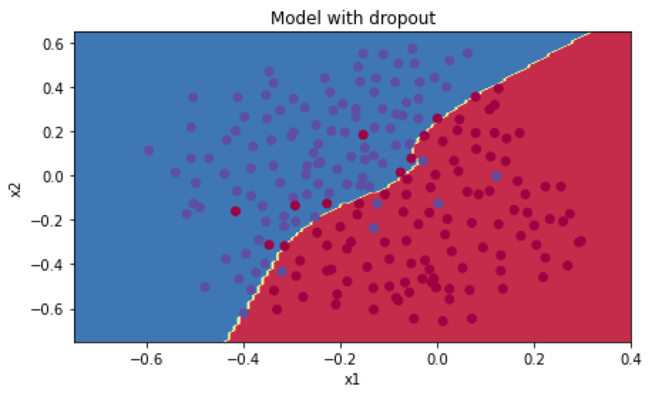
plt.title("Model with dropout")
axes = plt.gca()
axes.set_xlim([-0.75,0.40])
axes.set_ylim([-0.75,0.65])
plot_decision_boundary(lambda x: predict_dec(parameters, x.T), train_X, train_Y)
|
dropout正则化在训练集的预测准确率为0.929,测试集的准确率为0.95。分类图如下:
因为有部分公式可能因为博客插件不支持的原因,完整的笔记请看:
https://github.com/caixiongjiang/deep-learning-computer-vision
最后修改于 2022-07-20

本作品采用
知识共享署名-非商业性使用-相同方式共享 4.0 国际许可协议进行许可。