《数字图像处理》第二章—

《数字图像处理》第二章——图像压缩

图像压缩基本概念

压缩比： Cr = n1 / n2
相对数据冗余： Rd = 1 - 1 / Cr
无损压缩：压缩编码冗余和像素冗余称为无损压缩

图像压缩标准（包括视频）

主流的静态图像压缩标准（JPEG家族）：JPEG, JPEG-LS(无损压缩), JPEG-2000
主流的视频压缩标准（MPEG家族）：MPEG-1, MPEG-2, MPEG-3, MPEG-4 AVC

图像压缩的流程

以JPEG的压缩流程为例：

输入的图像——>图像分块——>映射器——>量化器——>编码器
                      解码器——>反映射——>输出图片

量化器是该过程中唯一对图像质量有损耗的

JPEG压缩

编码器

JPEG使用的是哈夫曼编码，哈夫曼编码得到的是一种无前缀编码，这会使得出现概率越高的元素编码长度越短，出现概率越低的元素编码长度越长，最后总的编码长度编程最短

哈夫曼编码使用规则：

1.每次取集合中最小的两个值，相加之后再加入原有的集合，再重复取最小的两个值，到最后只剩一个元素
2.将原有集合的数字进行编码，层数越高，编码长度越短

在JPEG中应用为：对像素出现的概率高低进行编码！

demo：

a1 - 0.4
a2 - 0.3
a3 - 0.1

对应编码：
a1 - 1
a2 - 01
a3 - 00

编码熵：$ -\sum_{i = 1}^n p(s)log_2^{p(s)}$ （概率*对应的自信息）

图像分块

在JPEG中采用8✖️8的小块进行分别处理，这么做的原因是分别对小块进行处理比对整张图像进行处理更加高效、

若JPEG为RGB的彩色图像，我们需要先将RGB通道转化为YCbCr通道，再对每个通道进行分块处理

模式“RGB”转换为“YCbCr”的公式如下：

Y= 0.257R+0.504G+0.098B+16
Cb = -0.148R-0.291G+0.439B+128
Cr = 0.439R-0.368G-0.071*B+128

python 中的PIL Image 本身是带有rgb2ycbcr()函数的，但是其MATLAB实现上有差异。

python中的自带函数实现：

1
2
3


from PIL import Image
image =Image.open("test.jpg")
image_ycbcr =image.convert("YCbCr")

python 实现MATLAB中rgb2ycbcr()函数：

 1
 2
 3
 4
 5
 6
 7
 8
 9
10
11
12
13
14


mat = np.array(
    [[65.481, 128.553, 24.966],
     [-37.797, -74.203, 112.0],
     [112.0, -93.786, -18.214]])
mat_inv = np.linalg.inv(mat)
offset = np.array([16, 128, 128])


def rgb2ycbcr(rgb_img):
    ycbcr_img = np.zeros(rgb_img.shape)
    for x in range(rgb_img.shape[0]):
        for y in range(rgb_img.shape[1]):
            ycbcr_img[x, y, :] = np.round(np.dot(mat, rgb_img[x, y, :] * 1.0 / 255) + offset)
    return ycbcr_img

JPEG映射器

首先了解一下，图像矩阵映射之后的误差如何衡量：

误差的指标为均方根误差(假设矩阵为M×N)： $$ MSE = \sqrt{\frac{1}{MN}\sum_{i = 1}^n\sum_{i = 1}^n(\dot{f}(x,y) - f(x,y))} $$

JPEG默认的映射器是做离散余弦变换（DCT），这里讲两种，第一种为K-L变换，第二种就是DCT变换。

K-L变换：将8×8矩阵的64个像素取1个进行K-L变换，然后进行反变换，计算均方误差，只传输均方误差最小的像素。（而对于K-L变换来说，第一个像素就是你需要传输的那个像素）

优缺点：优点就是传输的大小缩小了很多，缺点是需要根据具体的图像来确定映射矩阵

DCT变换：同K-L变换相似，它的矩阵是固定的。

DCT变换公式(二维离散n×n)： $$ T(u,v)=\sum_{x = 0}^{n - 1}\sum_{y = 0}^{n - 1}f(x,y)r(x,y,u,v) $$

逆变换： $$ f(x,y)=\sum_{u = 0}^{n - 1}\sum_{v = 0}^{n - 1}T(u,v)s(x,y,u,v) $$

其中： $$ r(x,y,u,v) = s(x,y,u,v) = \alpha(u)\alpha(v)cos{\frac{(2x+1)u\pi}{2n}}cos{\frac{(2y+1)v\pi}{2n}}$$ $$ \alpha(u) = \begin{cases} \sqrt{\frac{1}{n}} & {u = 0} \ \sqrt{\frac{2}{n}} & {u \neq 0} \end{cases}$$ $$ \alpha(v) = \begin{cases} \sqrt{\frac{1}{n}} & {v = 0} \ \sqrt{\frac{2}{n}} & {v \neq 0} \end{cases}$$

DCT优势：

1.其图像转换的矩阵是不变的

2.其良好的周期性

JPEG中的量化

JPEG采用的是均匀量化，假设量化因子为16，其量化的过程就是原图像处以16向下取整再乘以16。（量化因子越大，损耗越大）

需要注意的是：量化是按照右上到左下的锯齿状进行的，当JPEG进行到某一个系数时，发现后续量化后都变成了0，我们只需要用一个信号来表明结束

Max-Lloyd最优量化器：根据不同的图片个性定制量化方式

JPEG-LS（无损压缩）

无损压缩的编码思想：根据原像素矩阵进行预测，再与真实值比较，将产生的误差进行哈夫曼编码

解码：先用哈夫曼解码，在预测值上加上误差（有正有负），还原图像

两种预测方式：

$$F(x,y) = F(x - 1, y)$$
$$F(x,y) = \frac{F(x - 1, y) + F(x - 1, y - 1) + F(x, y - 1)}{3}$$

游程编码

一般用于编码二值图像！

demo：只有两种灰度值的图片，可以对每行每种灰度值连续出现的值和次数进行编码。（也就是相同灰度值所占行程的长度）

实验作业

本次实验作业全部用python3完成

第一题

JPEG的基本实现：
1.图像分成8×8的块
2.DCT变换
3.采用均匀量化（系数为N）
4.将图像进行逆DCT变换
5.可视化图像

代码如下：

 1
 2
 3
 4
 5
 6
 7
 8
 9
10
11
12
13
14
15
16
17
18
19
20
21
22
23
24
25
26
27
28
29
30
31
32
33
34
35
36
37
38
39
40
41
42
43
44
45
46
47
48
49
50
51
52
53
54
55
56
57
58
59
60
61
62
63
64
65
66
67
68
69
70
71
72
73
74
75
76
77
78
79
80
81
82
83
84
85
86
87
88
89
90
91
92


import matplotlib.pyplot as plt
import numpy as np
from PIL import Image


# 生成DCT矩阵
def func1(block_size):
    dct_matrix = np.zeros((block_size, block_size))
    for i in range(block_size):
        for j in range(block_size):
            if i == 0:
                a = np.sqrt(1 / block_size) #a代表转化系数
            else:
                a = np.sqrt(2 / block_size)
            temp = ((2 * j + 1) * i * np.pi) / (2 * block_size) #公式 cos(((2x + 1)u派)/2n)
            dct_matrix[i, j] = a * np.cos(temp) # 离散余弦变换
    return dct_matrix

# 按照指定块大小进行DCT变换
def func2(image, dct_mat):
    block_size = dct_mat.shape[0]
    height, width = image.shape
    dct_img = np.zeros((height, width), dtype=np.float32)
    for row in np.arange(0, height, block_size):
        for col in np.arange(0, width, block_size):
            block = np.array(image[row:(row + block_size), col:(col + block_size)], dtype=np.float32)
            dct_img[row:(row + block_size), col:(col + block_size)] = np.matmul(np.matmul(dct_mat, block), dct_mat.T)

    return dct_img


# 量化每个块 采用简单的除以side再乘以side，这里side取16
# 当side大于50时，图片量化损耗较大
def func3(dct_image, side):
    m, n = dct_image.shape
    for row in range(m):
        for col in range(n):
            a = dct_image[row, col]
            a /= side
            # 四舍五入
            if (int(a + 1) - a) < (a - int(a - 1)):
                dct_image[row, col] = int(a + 1) * side
            else:
                dct_image[row, col] = int(a - 1) * side

    return dct_image

# 逆DCT变换
def func4(image, dct_mat):
    block_size = dct_mat.shape[0]
    height, width = image.shape
    inv_dct_img = np.zeros((height, width), dtype=np.float32)
    for row in np.arange(0, height, block_size):
        for col in np.arange(0, width, block_size):
            block = np.array(image[row:(row + block_size), col:(col + block_size)], dtype=np.float32)
            inv_dct_img[row:(row + block_size), col:(col + block_size)] = np.matmul(np.matmul(dct_mat.T, block),
                                                                                    dct_mat)

    return inv_dct_img

def main(img_path):

    # 第一题实现
    src1 = np.array(Image.open(img_path).convert("L"))
    dct = func1(8)
    dct_img1 = func2(src1, dct)
    inv_dct_img1 = func4(dct_img1, dct)
    dct_img2 = func3(dct_img1, 16)
    inv_dct_img2 = func4(dct_img2, dct)

    # 重新导入图像（量化会对原图像进行修改）
    src = np.array(Image.open(img_path).convert("L"))

    img_list = [src, inv_dct_img1, inv_dct_img2]
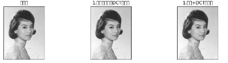
    img_name = ["原图像", "1.没有量化直接DCT的结果", "1.量化+DCT的结果"]

    plt.rcParams['font.sans-serif'] = ['SimHei']
    plt.rcParams['axes.unicode_minus'] = False

    _, axs = plt.subplots(1, 3, figsize=(12, 12))

    for i in range(1):
        for j in range(3):
            axs[i][j].imshow(img_list[i * 3 + j], cmap='gray', vmin=0, vmax=255)
            axs[i][j].set_title(img_name[i * 3 + j])
            axs[i][j].axes.get_xaxis().set_visible(False)
            axs[i][j].axes.get_yaxis().set_visible(False)

    plt.show()

if __name__ == '__main__':
    main('/Users/jarsonsmac/Desktop/学习资料/数字图像处理和机器视觉/week2/woman.jpg')

实验结果：第一题实验结果

第二题

直接对原始图像进行量化

代码如下：

 1
 2
 3
 4
 5
 6
 7
 8
 9
10
11
12
13
14
15
16
17
18
19
20
21
22
23
24
25
26
27
28
29
30
31
32
33
34
35
36
37
38
39
40
41
42
43
44
45
46
47
48
49
50
51


import matplotlib.pyplot as plt
import numpy as np
from PIL import Image

# 量化每个块 采用简单的除以side再乘以side，这里side取16
# 当side大于50时，图片量化损耗较大
def func3(dct_image, side):
    m, n = dct_image.shape
    for row in range(m):
        for col in range(n):
            a = dct_image[row, col]
            a /= side
            # 四舍五入
            if (int(a + 1) - a) < (a - int(a - 1)):
                dct_image[row, col] = int(a + 1) * side
            else:
                dct_image[row, col] = int(a - 1) * side

    return dct_image

def main(img_path):

    # 第三题实现
    src3 = np.array(Image.open(img_path).convert("L"))
    image3 = func3(src3, 16)
    src4 = np.array(Image.open(img_path).convert("L"))
    image4 = func3(src4, 50)

    # 重新导入图像（量化会对原图像进行修改）
    src = np.array(Image.open(img_path).convert("L"))

    img_list = [src, image3, image4]
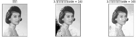
    img_name = ["原图像", "3.直接量化的结果(side = 16)", "3.直接量化的结果(side = 50)"]

    plt.rcParams['font.sans-serif'] = ['SimHei']
    plt.rcParams['axes.unicode_minus'] = False

    _, axs = plt.subplots(1, 3, figsize=(12, 12))

    for i in range(1):
        for j in range(3):
            axs[i][j].imshow(img_list[i * 3 + j], cmap='gray', vmin=0, vmax=255)
            axs[i][j].set_title(img_name[i * 3 + j])
            axs[i][j].axes.get_xaxis().set_visible(False)
            axs[i][j].axes.get_yaxis().set_visible(False)

    plt.show()


if __name__ == '__main__':
    main('/Users/jarsonsmac/Desktop/学习资料/数字图像处理和机器视觉/week2/woman.jpg')

实验结果：第二题实验结果

第三题

计算给定直方图及预测其误差

共有两种预测方式：

1.$$F(x,y) = F(x - 1, y)$$

2.$$F(x,y) = \frac{F(x - 1, y) + F(x - 1, y - 1) + F(x, y - 1)}{3}$$

代码如下：

 1
 2
 3
 4
 5
 6
 7
 8
 9
10
11
12
13
14
15
16
17
18
19
20
21
22
23
24
25
26
27
28
29
30
31
32
33
34
35
36
37
38
39
40
41
42
43
44
45
46
47
48
49
50
51
52
53
54
55


# 第一种预测方案
def forecast1(matrix):
    m, n = matrix.shape
    fore_mat = np.zeros((m, n), dtype=np.int32)
    dif_sum = 0
    for i in range(m):
        for j in range(n):
            if(i == 0):
                fore_mat[i][j] = matrix[i][j]
            else:
                fore_mat[i][j] = matrix[i - 1][j]
            dif_sum += abs(fore_mat[i][j] - matrix[i][j])

    return dif_sum


# 第二种预测方案
def forecast2(matrix):
    m, n = matrix.shape
    fore_mat = np.zeros((m, n))
    dif_sum = 0
    dir = np.array([[-1, 0], [-1, -1], [0, -1]]) #上 左上 左
    for i in range(m):
        for j in range(n):
            sum = 0
            cnt = 0
            for k in range(3):
                dx = i + dir[k][0]
                dy = j + dir[k][1]
                if dx < 0 or dy < 0:
                    continue
                sum += matrix[dx][dy]
                ++cnt
            if sum == 0 or cnt == 0: #被除数不能为0和除数不能为0
                fore_mat[i][j] = 0
            else:
                fore_mat[i][j] = sum / cnt
            dif_sum += abs(fore_mat[i][j] - matrix[i][j])
    return dif_sum

def main():
    # 第5题实现
    im2 = Image.open("/Users/jarsonsmac/Desktop/学习资料/数字图像处理和机器视觉/week2/woman.jpg")
    src7 = np.array(im2.convert("L"))  # 图像转化为矩阵
    dif1 = forecast1(src7)
    dif2 = forecast2(src7)
    print("第一种预测方法的墒=" + str(dif1))
    print("第二种预测方法的墒=" + str(dif2))
    if dif1 < dif2:
        print("第一种预测方法好，墒低")
    else:
        print("第二种预测方法好，墒低")

if __name__ == '__main__':
    main()

实验结果：

第一种预测方法的墒=2726550
第二种预测方法的墒=86114089.0
第一种预测方法好，墒低

最后修改于 2022-02-28

本作品采用知识共享署名-非商业性使用-相同方式共享 4.0 国际许可协议进行许可。